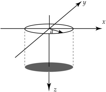
Figure 1: Illustration of a baffled transducer.
THE DREAM (Discrete REpresentation Array Modeling) toolbox is an open source software, released under the GNU General Public License (GPL), for both Matlab and Octave for simulating acoustic fields radiated from common ultrasonic transducer types and arbitrarily complicated ultrasonic transducers arrays. The DREAM toolbox enables analysis of beam steering, beam focusing, and apodization for wide band (pulse) excitation both in near and far fields. The toolbox is also provided with a user friendly graphical user interface (GUI).
The toolbox consists of a set of routines for computing (discrete) spatial impulse response (SIRs) for various single-element transducer geometries as well as multi-element transducer arrays. Based on linear systems theory, these SIR functions can then be convolved with the transducer’s electrical impulse response to obtain the acoustic field at an observation point. Using the DREAM toolbox one can simulate ultrasonic measurement systems for many configurations including phased arrays and measurements performed in lossy media.
The DREAM toolbox uses a numerical procedure based on based on the discrete representation (DR) computational concept [1, 2] which is a method based on the general approach of the spatial impulse responses [3, 4].
THE DREAM toolbox is an open source software and the source code for the toolbox is freely redistributable under the terms of the GNU General Public License (GPL) as published by the Free Software Foundation (http://www.gnu.org). See also the file COPYING which is distributed with the DREAM Toolbox.
The DREAM Toolbox can be downloaded at: http://www.signal.uu.se/Toolbox/dream/. At this website you can also find information how to contact the authors and report bugs etc.
The DREAM toolbox is distributed in the hope that it will be useful but WITHOUT ANY WARRANTY. More specifically:
THE PROGRAM IS PROVIDED “AS-IS” WITHOUT WARRANTY OF ANY KIND, EITHER EXPRESS OR IMPLIED, INCLUDING BUT NOT LIMITED TO THE IMPLIED WARRANTIES OR CONDITIONS OF MERCHANTABILITY OR FITNESS FOR A PARTICULAR PURPOSE. IN NO EVENT SHALL ANY OF THE AUTHORS OF THE DREAM TOOLBOX AND/OR THE DEPARTMENT OF ENGINEERING SCIENCES AT UPPSALA UNIVERSITY, SWEDEN, OR THE INSTITUT D’ELECTRONIQUE ET DE MICRU-ELECTRONIQUE DU NORD (IEMN-DOAE-UMR CNRS 9929), ECOLE CENTRALE DE LILLE, FRANCE, BE LIABLE FOR ANY SPECIAL, INCIDENTAL, INDIRECT, OR CONSEQUENTIAL DAMAGES OF ANY KIND, OR DAMAGES WHATSOEVER RESULTING FROM LOSS OF USE, DATA, OR PROFITS, WHETHER OR NOT THE AUTHORS OF THE DREAM TOOLBOX HAVE BEEN ADVISED OF THE POSSIBILITY OF SUCH DAMAGES, AND/OR ON ANY THEORY OF LIABILITY ARISING OUT OF OR IN CONNECTION WITH THE USE OR PERFORMANCE OF THIS SOFTWARE.
THE DREAM Toolbox can be installed both using pre-compiled binaries and from source code. Binaries are currently available for Linux (x86/x86_64), Windows (x86), and for Intel Macs (Mac OS X). The binaries are compiled using generic compiler flags and without support for the fftw library (for the transducer functions) and should, therefore, run on most setups.
If you want higher performance then it is recommended that you compile DREAM from source. There is a bash script and m-files included in the source distribution to facilitate building the toolbox and, furthermore, the Makefiles used in build process can easily be edited for further fine tuning of the performance.
Note: since the oct-API often changes between releases of Octave the binaries will probably only work for the version of Octave that they were compiled for. For this reason binaries for Octave are no longer available and you need to install the toolbox from source which easily can be done with the Octave pkg command (see Section 4.4).
If you want to use the parallel (threaded) DREAM functions you need to install the Pthreads-Win32 library.
Download the library from: http://sourceware.org/pthreads-win32/ and put the
pthreadGC2.dll file in a suitable directory, such as,
C:WINDOWSSystem32;
this file is now also available on the DREAM web page. If you want to build the Pthreads library for Windows
from source then you can find instructions in Appendix A.
The fftconv_p and sum_fftconv_p use the FFTW3 library (see Section 10.3). A Windows version of this library can be found at: http://www.fftw.org/install/windows.html but it is now also available on the DREAM web page. Copy the libfftw3-3.dll file to C:WINDOWSSystem32. If you want to build the FFTW library for Windows from source then you can find instructions in Appendix B.
To install DREAM for Octave on Windows see Sections 4.5.4 and 4.5.5.
The fftconv_p and sum_fftconv_p functions use the FFTW3 library (see Section 10.3). Instructions for installing fftw on MacOS X can be found at:
http://www.fftw.org/install/mac.html
As mentioned above, the DREAM Toolbox must be installed from sources for Octave. Recent versions of Octave have a package manager tool (pkg) for that purpose. Given that you have the developer tools for your system installed (for Windows see Sections 4.5.4 and 4.5.5) you should be able to install DREAM by,
You should now be able to see the DREAM packege by typing:
at the Octave command line.
To build the DREAM Toolbox from sources you need to have developer tools installed for your system (compiler, linker, etc.). Start with downloading (and uncompressing) the (full) source DREAM-2.x.x.tgz file. This file contains the source code, the documentation (the user manual), and the html code for the web pages. The build process is based on Makefiles both for C/C++ code and for building the (LATEX) user manual and html documentation. Therefore, to build the documentation you need to have TEX/LATEX installed and, furthermore, to build the html documentation you also need the tex4ht and highlight tools.5
There are three methods that can be used to build the DREAM Toolbox on unix from sources. The first, and simplest, is to use the m-script build_mexfiles_unix.m, the second is to use the bash script build_dream.sh and the third is to manually edit the build configuration file Make.inc and then compile the sources.
Method 1: Using the build_mexfiles_unix.m script.
This is the simplest method but there is no optimization for the used architecture and the attenuation code is build without fftw support (see Section 4.5.8). This will also only build the mex-files (not the oct-files).
file (the DREAM sources contain C++ style comments and they will not compile with -ansi).
Method 2: Using the build_dream.sh bash script.
The bash script build_dream.sh will probe the machine for cpu, architecture (32 or 64 bits) and then use a pre-defined set of compiler flags for the machine (currently only x86 is supported). This script will both build the mex-/oct-interfaces and the documentation for DREAM. It is assumed that Matlab is installed in /usr/local/matlab. If you have installed Matlab somewhere else then you can create a symbolic link to the /usr/local/matlab dir. Usage:
Then add your DREAM install directory to the Matlab/Octave path(s). That is, add
addpath(’/your_installation_dir/’) to your matlab/startup.m file and/or .octaverc file.
Method 3: Manual configuration.
There is currently only one method to build the DREAM mex-files for MacOS X and that is to use the build_mexfiles_unix.m script (the Makefiles do not currently work under Mac OS X).
file (the DREAM sources contain C++ style comments which will not compile with -ansi).
Method 1: Using the MinGW/Gnumex Tools.
Method 2: Using the MSVC 2008 Express Edition
Method 3: Matlab’s build-in LCC compiler (depreciated).
Note the LCC compiler, at least LCC for Matlab R2007b, cannot build the parallel mex-functions since the compiler cannot parse the Pthread-Win32 header files. All parallel functions will, therefore, be unavailable if you are using the LCC compiler.
The pkg source can be build also on Windows with resent versions of Octave (tested with Octave 3.2.3 [MinGW 4.4.0]). To do this, using the native Windows Octave from octave-forge, you only need to install Octave since fftw, the MinGW compiler, and the pthread libs are included in the Octave package).
This section describes how to build the DREAM oct-files for Windows using the MSVC compiler. But note that, as of spring 2009, Octave binaries build with the MSVC compiler are no longer available at octave-forge due to license issues. It is therefore recomended that the MinGW compiler is used instead as described in Section 4.5.4! To use MSVC one therefore needs an older MSVC build binary of Octave or one has to build Octave (and all its dependencies) using the MSVC compiler and then follow the procedure below:
to the file (change the path to the actual version of Octave that you use).
If you have an older 64-bit Matlab installation (eg. 2007x) then follow these steps:
If you have Matlab 2008b, or above,8
then read and follow the instructions in Mathworks FAQ:
http://www.mathworks.fr/support/solutions/en/data/1-6IJJ3L/index.html?solution=1-6IJJ3L. Then
run the build_mexfiles_windows.m script.
Currently there is no support for building 64-bit oct-files since there is no 64-bit version of Octave for Windows available (yet).
The attenuation code in the DREAM Toolbox uses FFTs extensively. To speed up the FFT computations (by 10% to 50%) one can compile The DREAM Toolbox with FFTW support for the attenuation code. To do this you need to compile all functions with the flag -DUSE_FFTW and link with -lfftw3. This can be accomplished by changing:
to
in the file Make.default before compiling the toolbox if you are using Method 3 described in Section 4.5.1 (the build_dream.sh uses fftw by default).
THE impulse response method is an approach based on linear systems theory to model acoustic fields from ultrasonic transducers; the method was introduced by Tupholme and Stepanishen in the late 60’s, early 70’s [3, 4]. The impulse response method is based on linear acoustics and can be used to model acoustic fields and (double-path) responses for both single transducer setups and for array imaging. The idea is to divide the imaging system in two parts: the first one accounts for acoustical wave propagation effects (i.e., the diffraction effects) from the transducer surface to the observation point, and the second one accounts for the electro-acoustical effects. These two parts are then convolved to obtain a model for the total imaging system.
The impulse response method is very flexible since, (i) by linearity the response from multi-element transducers (such as array transducers) can be obtained be means of super-position and (ii) arbitrary input signals can be treated by simply convolving the electro-acoustical impulse response with the input signal. In this section we will present a short introduction to the impulse response method and, in particular, discuss how to use the method for discrete-time modeling.
The impulse response method is based on the assumption that the transducer can be treated as a baffled piston. This assumption implies that we only need to consider the active area of the transducer when modeling the wave propagation. That is, if the source (the transducer) is located in the rigid plane, often referred to as the rigid baffle as illustrated in Figure 1, then the baffle () will not contribute to the field.
The pressure at an observation point is then described by the Rayleigh integral
| (1) |
where it is where we for simplicity have assumed that the normal velocity is uniform on the transducer’s surface . The Rayleigh integral formula (1) simply states that the acoustic field at an observation point is the sum of the contributions from all points of the active area of the transducer. The impulse response in Eq. (1) is usually referred to as the (forward) spatial impulse response (SIR).
The normal velocity, , depends on both the input signal, , and the electro-acoustical properties of the transducer, which can be described with the (forward) electrical impulse response . Thus, the pressure at can be expressed by the convolutions of the input signal and the two (forward) impulse responses according to,
| (2) |
Double-path (pulse-echo) responses can be treated in a similar way by convolving the forward response (2) with the backward electrical (acousto-electrical) response and the backward SIR for a point source at .
Analytical solutions to SIRs exist for a few geometries, but one must in general resort to numerical methods. Also, these time continuous solutions are normally not practical since all acquired signals (the data) are normally sampled and time discrete models are, therefore, needed; sampling of time continous SIRs is discussed in Section 5.2.
Before we discuss sampled SIRs, and the particular method use by the DREAM Toolbox, let us consider a case where there exist an analytical solution.
Example 1 (The SIR for a Circular Disc). The SIR of a circular disc (see illustration in Figure 2) has an analytical solution [4]
which can be divided in two cases: (i) when the observation point is inside the aperture of the disc , where is the transducer radius, and (ii) when the observation point is outside the aperture. The disc is assumed to be located in the – plane centered at . If we let denote the distance in the – plane from the center axis of the disc to the observation point, , then the circular disc SIR is given by
| (3) |
where is the earliest time that the wave reaches the observation point when , , and are the propagation times corresponding to the edges of the disc that are closest and furthermost away from , respectively.
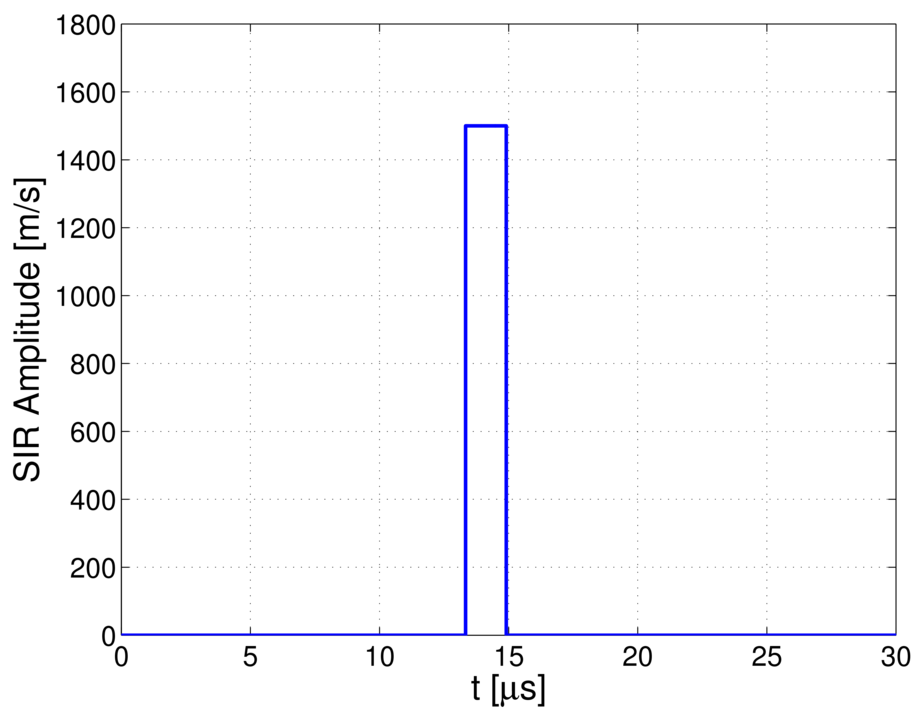
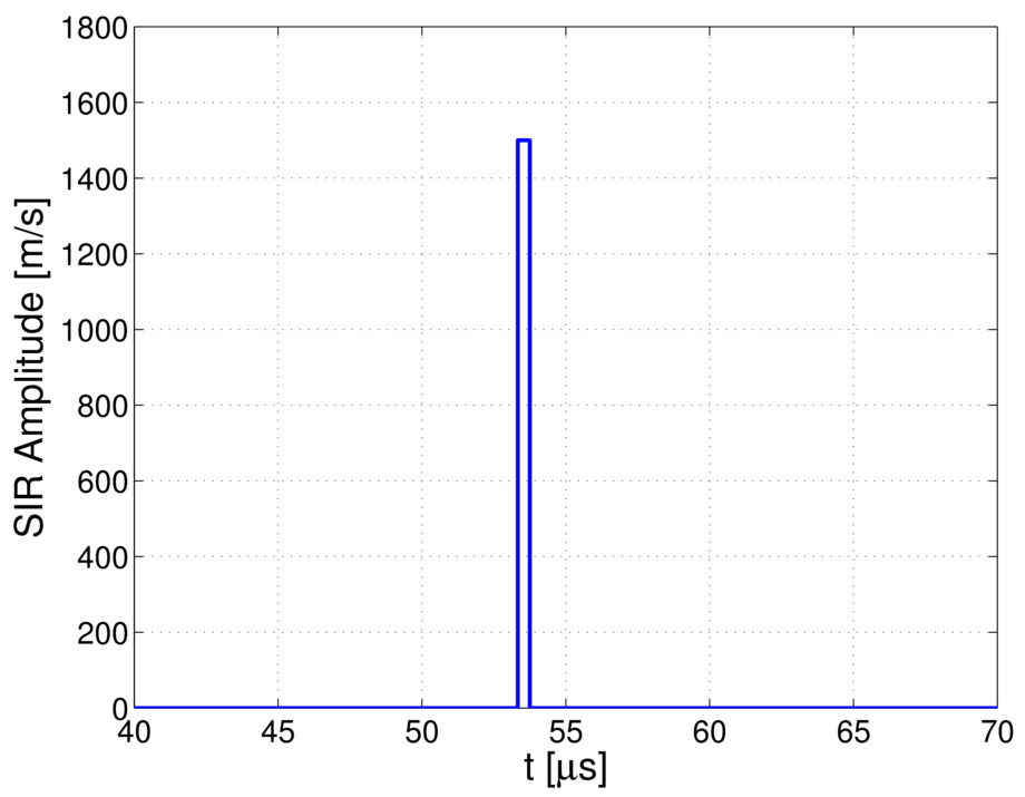
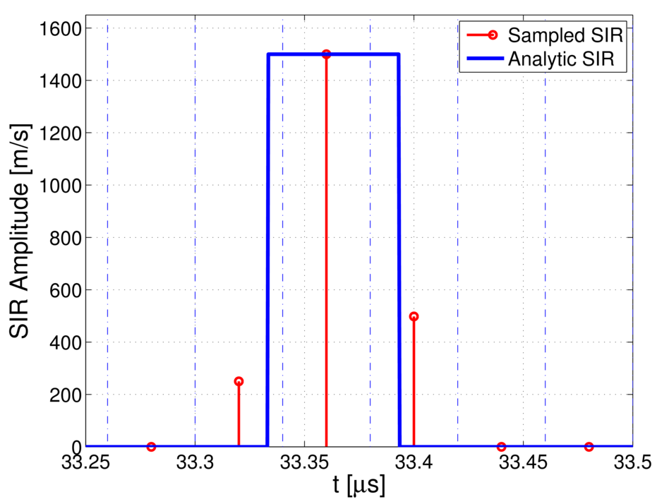
Noticeable is that the pulse amplitude of the on-axis SIR is constant regardless of the distance to the observation point.9 The duration of the on-axis SIR is given by at . As the distance increases the duration, , of the SIR becomes shorter, and for large it approaches to the delta function. The transducer size effects are therefore most pronounced in the near-field. This is illustrated in Figure 3 where the on-axis SIRs at and mm, respectively are shown.
The duration at is longer than that of and if the distance, , increases then the on-axis SIR will approach to a delta function, cf. Figures 3(a) and (b).
As mentioned above, there exist no analytical analytical solutions for many transducer geometries, and in such situations numerical methods must be used. The DREAM Toolbox uses a method based on the discrete representation (DR) computational concept [1, 2]. The DR method is very flexible in the sense that complex transducer shapes as well as arbitrary focusing methods easily can be modeled. Another benefit of the DR method is that the SIRs are directly computed in a discrete form which is convenient since this directly allows for digital signal processing. The DR method is described in Section 5.3 below, but first we will discuss sampling of spatial impulse responses.
Before we introduce the discrete representation (DR) method, which the DREAM toolbox transducer functions are based on, let us discuss sampling of spatial impulse responses. This is of interest since our ultimate goal normally is to model the total sampled imaging system which includes both acoustic propagation effects (the SIRs) as well as input signals and electro-acoustical effects.
To obtain a discrete model we need a discrete representation of the SIRs. That is, the analytical expressions for the SIRs discussed in Section 5.1 must be converted to a discrete form in order to be useful for digital signal processing; a proper discrete representation of the SIRs is necessary so that when the sampled SIR is convolved with the normal velocity the resulting waveform can faithfully represent the sampled measured waveform.
The analytical SIRs have an infinite bandwidth due to the abrupt amplitude changes that, for example, could be seen in the line and disc solutions above. In some situations the duration of a SIR may even be shorter than the sampling interval, , and it is therefore not sufficient to simply sample the analytical SIRs by simply taking the amplitude at the sampling instants since the SIR may actually be zero those time instants. The SIRs are however convolved with a band-limited normal velocity signal, hence the resulting pressure waveform must also be band-limited, cf. (2). Consequently, we only need to sample the SIR in such way that the band-limited received A-scans are properly modeled.
In a sampled system the impulse responses are given at discrete time instants, (given by the sampling period ) and to faithfully represent the SIRs we need to collect all contributions from the continuous time SIRs in the corresponding sampling interval . A discrete version of the a time continuous SIR is then obtained by summing all contributions from the SIR in the actual sampling interval. That is, the sampled SIR is defined as
| (4) |
The division by retains the same unit (m/s) of the sampled SIR as the continuous one. The amplitude of the sampled SIR, at time , is then the mean value of the continuous SIR in the corresponding sampling interval, . Also, as seen from the analytical solutions above, the SIRs always have a finite length as the transducer has a finite size. The sampled SIRs are therefore naturally represented by finite impulse response filters (FIRs).
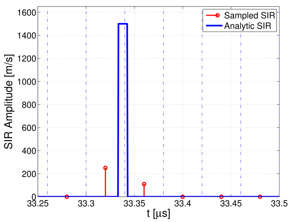
The effect of the sampling scheme (4) is illustrated in Figure 4 for two discs with radii 1.2 and 3 mm, respectively, where the sampling interval, , was 0.04s.
(a) Continuous and sampled spatial impulse responses of a
circular disc with radius
mm. |
(b) Continuous and sampled spatial impulse responses of a
circular disc with radius
mm. |
In Figure 4(a) the analytic SIR is shorter than the sampling interval, . The max amplitude of the discrete SIR is therefore lower than then the max amplitude of the continuous SIR. If the duration of the analytic SIR is longer than the sampling interval, as for the 3 mm disc shown in Figure 4(b), then the max amplitudes of the on-axis sampled and analytic disc SIRs will be the same.
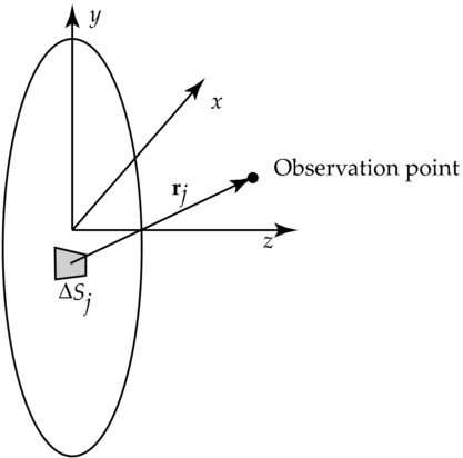
As mentioned in previous in Section 5.1 the analytical spatial impulse responses are only available for a few simple transducer geometries. Therefore, for a transducer with an arbitrary geometry a numerical method must be used. The numerical method used in this toolbox is based on the discrete representation (DR) method, which is based on a discretization of the Rayleigh integral formula (1). In the DR method, the radiating surface is divided into a set of small surface elements (see illustration in Figure 5), and
the surface integral in the Rayleigh formula is replaced by a summation. The DR method facilitates computation of SIRs for non-uniform excitation, apodization of the aperture, and arbitrary focusing laws since each surface element can be assigned a different normal velocity, apdodization or time-delay. The DR computational concept can therefore be used for computing SIRs for an arbitrary transducer shape or array layout [1, 2].
A discrete SIR, computed using the DR method, can be found by first dividing the total transducer surface into a set of surface elements . Second, let denote an aperture weight, and the distance from the th surface element to the observation point. The discrete SIR can now be approximated by
| (5) |
where is a user defined focusing delay and , for . The scaling factor
| (6) |
in (5) represents the amplitude of the impulse response for an elementary surface at excited by a Dirac pulse. Hence, the total response, at time , is a sum of contributions from those elementary surface elements, , whose response arrive in the time interval .
The accuracy of the method depends on the size of the discretization surfaces . It should, however, be noted that high frequency numerical noise due to the surface discretization is in practice not critical since the transducer’s electrical impulse response has a bandwidth in the low frequency range (for a further discussion see [2]). Also, these errors are small if the elementary surfaces, , are small. The DR-method is very flexible in the sense that beam steering, focusing, apodization, and non-uniform surface velocity can easily be included in the simulation.
The computational procedure for an attenuation free medium implies a Dirac-type Green’s function [1]. The discrete approach in the DREAM toolbox above is, however, also applicable to the problems characterized by an arbitrarily shaped causal Green’s function. In such a case a Dirac function is simply replaced by a sampled version of this function. This characteristic extends the field of applications and allows, for example, the computations for lossy media. For such a case, the free space Green’s function , where is a point in the transducer surface and is the observation point, should be replaced by its causal counterpart related to the medium with absorption. The solution for lossy media used in the DREAM toolbox for has the following frequency-domain form [1, 5]:
| (7) |
where
| (8) |
, and . The time-domain transfer function is then obtained by means of the inverse Fourier transform
| (9) |
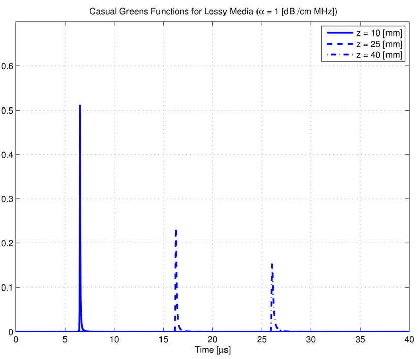
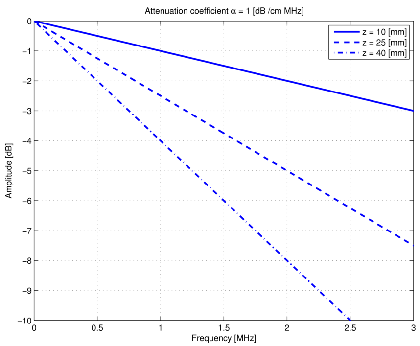
In the DREAM toolbox this computation is performed by a discrete Fourier transform for each surface element dxdy. An illustration of the effects due to lossy media for an attenuation of coefficient, of 1 [db/cm MHz] is shown in Figure 6 for 10 mm, 25 mm, and 40 mm respectively.
IN his section a quick start on how to perform simulations with DREAM is presented. Here only a simple example is shown just to illustrate what is needed to simulate an ultrasonic measurement system. We will use a circular transducers for this example but more advanced examples can be found on the DREAM web page http://www.signal.uu.se/Toolbox/dream/ on the Examples page. Also more details of the various functions in the DREAM Toolbox can be found in Sections 7, 8, and 10, respectively.
Let us study a the pressure response for a circular transducer using water as the propagation medium (with a sound speed [m/s]). We start by setting the sampling frequency and defining the points of interest, the so-called observation points. The observation points are located on a line at mm, from 1–50 mm with 1 mm between them:
Then we need to define the discretization parameters for both the transducer surface and the temporal sampling:
We must also define the sound speed of the medium, normal velocity, and attenuation. Here we choose an attenuation free medium () and a unit normal velocity:
The size of the transducer must also be defined, here we use a circular transducer with a 5 mm radius:
Finally we set the start point of the SIR and call the DREAM function dreamcirc to compute the discrete SIRs:
THE transducer functions are implemented as Matlab mex-functions and Octave oct-functions; a mex/oct-function is pre-compiled code that is dynamically linked to Matlab/Octave at run time. This greatly increases the computation speed compared to using ordinary m-files since the DR-concept (see [2]) uses for and while loops extensively. An overview of the transducer functions can be found in Table 1.
| Transducer type | DREAM function |
| Strip transducer | dreamline |
| Rectangular transducer | dreamrect |
| Focused rectangular transducer | dreamrect_f |
| Circular transducer | dreamcirc |
| Focused circular transducer | dreamcirc_f |
| Spherical concave transducer (focused) | dreamsphere_f |
| Spherical convex transducer (defocused) | dreamsphere_d |
| Cylindrical concave transducer (focused) | dreamcylind_f |
| Cylindrical convex transducer (defocused) | dreamcylind_d |
| Array with rectangular elements | dream_arr_rect |
| Array with circular elements | dream_arr_circ |
| Array with cylindrical concave elements (focused) | dream_arr_cylind_f |
| Array with cylindrical convex elements (defocused) | dream_arr_cylind_d |
| Annular array | dream_arr_annu |
By convention, a transducer function name ending with “_f” is a focused transducer (or has focused transducer elements) and a transducer function name ending with “_d” is defocused (convex) transducer.
The transducer functions can be divided in two groups, single transducer functions and array functions. The names of both groups starts with “dream” and the array functions are distinguished from single transducer functions by “_arr_”. Note that arbitrary arrays (with mixed forms of transducer elements) can be modeled using the single transducer functions and then adding their corresponding responses.
The transducer functions can compute SIRs for multiple observation points. The observation points are given by a matrix Ro were the first column contains the -coordinates, the second the -coordinates, and the third the -coordinates, respectively ( is the number of observation points).
The single element transducers are, by convention, all centered at and the SIRs are computed relative to this center point. The array functions uses a grid matrix G to define the positions of the array elements (see Section 7.4). The SIRs are therefore computed relative the positions given by the grid matrix for the arrays.
The four-element vector s_par = [dx dy dt nt] determines the spatial discretization and the temporal sampling properties. The spatial discretization of the transducer surface is given by dxdy; small values of dx and dy results in a finer mesh, and a higher numerical accuracy, compared to larger ones. The temporal sampling interval (or ) is given by dt and the length of the SIR-vector is determined by nt. If nt is chosen too low so that any non-zero component of the SIR is not within the time-window defined by [delay dt*(nt-1)+delay] an error message will be printed (See Section 7.1.3 for a description of the delay parameter and Section 7.1.6 for a description of the error handling in the DREAM toolbox).
The starting point of the SIR-vector(s) is given by the delay parameter delay ([s]). The delay parameter can either be a scalar, then all SIRs will have the same starting point, or it can be a vector with a length that must be equal to the number of observation points. In the latter case each observation point has a SIR with a different starting point.
The material parameters are given by the three-element vector m_par = [v cp alfa]:
Note: if alfa then the SIRs are compensated for attenuation. Note that the attenuation calculation involves a computation of an inverse discrete Fourier transform of length nt for every surface element dxdy [2] This results in a longer computation time compared to when alfa = 0. See also Section 10.2.
The focusing in the DREAM toolbox is controlled with the two parameters foc_met and focal. The foc_met parameters is a text string that selects the focusing method, options are:
This type of focusing is used for the two single transducer functions (dreamrect_f and dreamcirc_f see Section 7.3) and for the array functions (Section 7.5). The spherical and cylindrical transducer functions also use focusing but there focusing is controlled by a single parameter R (see Sections 7.3.6, 7.3.7, 7.3.8, and 7.3.9).
There are three levels of error reporting for the transducer functions. An error typically occur when the SIR do not fit within the time window, defined by the delay, sampling period, and length parameters. The levels are controlled by the optional err_level parameter which is a text string with the following alternatives:
The error message contains a number that tells how many samples outside the time window the SIR is. The default error level is ’stop’ (if the err_level is omitted).
The first output argument of transducer functions, H, is a matrix or vector, containing the spatial impulse response(s).
Each column H contain the SIR for the corresponding entry in the observation point input matrix Ro (see Section 7.1.1).
The second (optional) output argument, err, is negative if an error has occurred and 0 otherwise.
If, for example, err_level = ’ignore’ then no error message will be printed but err will be negative if an error occurred so the error can be detected. This is useful for displaying error dialog boxes in GUIs, for example.
As mentioned above all single element transducers are centered at . There is, however, no loss in generality since the response at other transducer positions can simply be obtained by offsetting the coordinate system after computation.
The line, or strip, transducer has a length a and a (small) thickness equal to dy (in s_par).
Syntax:
Geometrical parameters:
The size of the rectangular transducer is determined by a and b.
Syntax:
Geometrical parameters:
The size of the rectangular focused transducer is determined by a and b and the focusing is described in Section 7.1.5.
Syntax:
Geometrical parameters:
The size of the circular transducer is determined by the single parameter r.
Syntax:
Geometrical parameters:
The size of the focused circular transducer is determined by the parameter r and the focusing is described in Section 7.1.5.
Syntax:
Geometrical parameters:
Syntax:
Geometrical parameters:
Syntax:
Geometrical parameters:
Syntax:
Geometrical parameters:
Syntax:
Geometrical parameters:
The positions of the array transducer elements are determined by the grid matrix G. The first column contain the (center) -positions of the elements, the second the -positions, and the third the -positions ( is the number of elements), respectively. This approach is very flexible and allows for arbitrary array geometries that not is restricted to equally spaced linear or 2D arrays.
The array focusing has an extra option, ’ud’, compared to the focusing methods described in Section 7.1.5:
When user defined focusing is used the ’focal’ parameter is a vector of focusing delays (in s). Each element in ’focal’ then delays the signal to the corresponding element in the array (given by the grid matrix).
The beam steering in the DREAM toolbox is controlled by the two parameters steer_met and steer_par. The steer_met is a text string with four alternatives: ’off’, ’x’, ’y’, and ’xy’. The steer_par is a two-element vector steer_par = [theta phi] where theta [deg] is the x-direction steer angle and phi [deg] the y-direction steer angle.
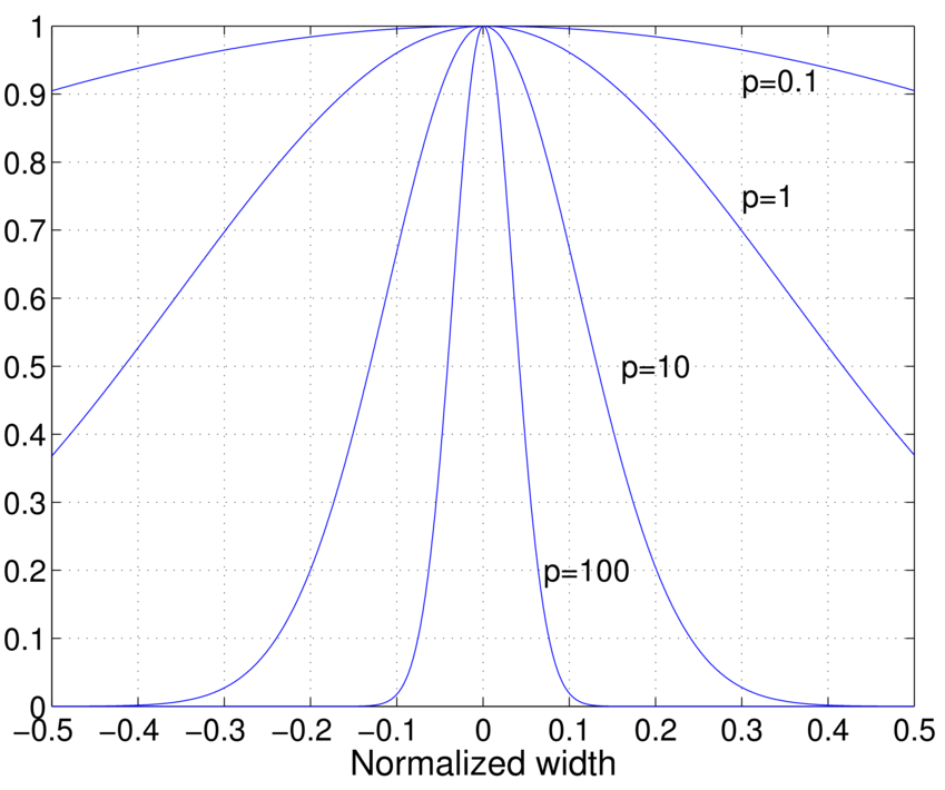
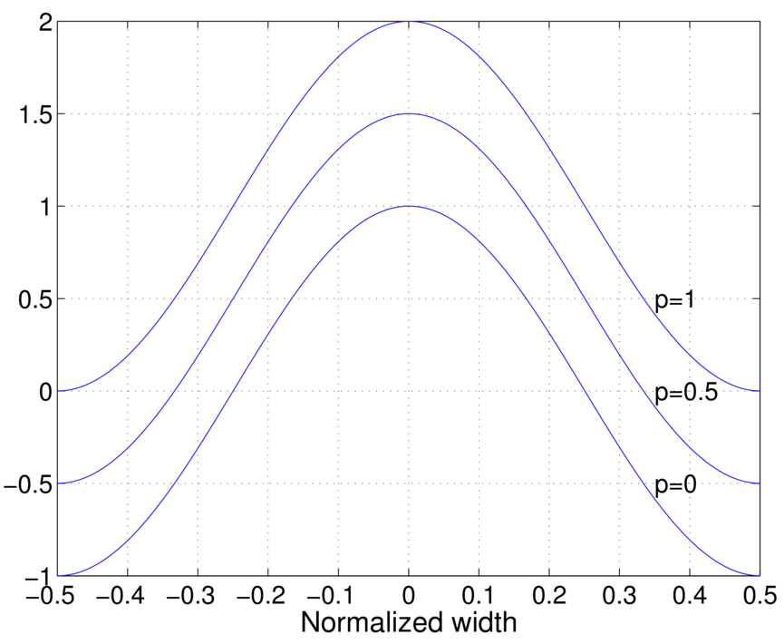
The DREAM toolbox has five pre-defined apodization windows that can be used for the array functions:
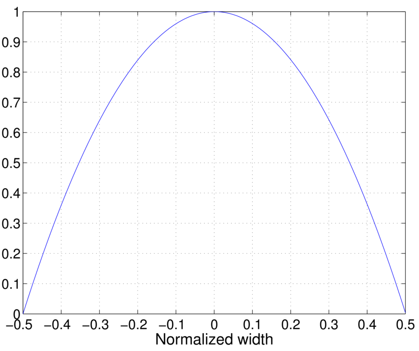
Additionally to the pre-defined apodizations one can have a user defined apodization weights. Figure 7 show some examples of these function.
There are three parameters that controls the apodization in the DREAM toolbox, apod_met, apod, and win_par. The apod_met parameter is string variable for selecting apodization method, options are:
The second parameter, apod, is a vector of apodization weights that is used for the ’ud’ option. Pass an empty matrix ([]) if one of the other options are used. The last parameter, win_par (scalar), is used for raised cosine and Gaussian apodization functions. See also Section 10.1.
Syntax:
Geometrical parameters:
Syntax:
Geometrical parameters: r - Radius of the transducer elements.
Syntax:
Geometrical parameters:
Example (linear array):
Syntax:
Geometrical parameters:
Syntax:
Geometrical parameters:
The first element in G is the radius of the center element; then G has two entries for each annulus (the inner and outer radius). Hence, the length of G must be odd for the annular array.
The apod_met parameter has the following entries for the annular array function:
Since the SIR computation for two different observation points is independent one can easily divide the observation points in sets and let a different process handle each set. On a multiprocessor machine, where each process (or thread) can run on a separate CPU simultaneously, this will speed up the computations. In the DREAM toolbox this is performed using (POSIX) threads; the SIRs for each set is computed in its own thread.The DREAM functions with thread support has an extra parameter n_cpus and a “_p” in its function name. For example, to compute SIRs for a rectangular transducer on 2 CPUs use:
where n_cpus is an integer . To see if the two threads are running using Linux, open new terminal window and use the command top. You should see something like:
As one can see there are two Matlab processes running on 99.9% instead on just one. Note that there is an overhead when creating (and running) new threads. If the distributed computations are very short the computations may not be faster for the parallel algorithm than the serial. On uni-processor computers the thread enabled functions may be slower than the non-threaded functions due to this overhead (if the hardware and software do not support hyper threading).
The functions currently available with parallel (thread) support is shown in Table 2.
| Transducer type/operation | DREAM function | Linux | Mac | Windows |
| Strip transducer | dreamline_p | Yes | Yes | Yes (see Sec. 4.2) |
| Rectangular transducer | dreamrect_p | Yes | Yes | Yes (see Sec. 4.2) |
| Focused rectangular transducer | dreamrect_f_p | Yes | Yes | Yes (see Sec. 4.2) |
| Circular transducer | dreamcirc_p | Yes | Yes | Yes (see Sec. 4.2) |
| Focused circular transducer | dreamcirc_f_p | Yes | Yes | Yes (see Sec. 4.2) |
| Spherical concave transducer | dreamsphere_f_p | Yes | Yes | Yes (see Sec. 4.2) |
| Spherical convex transducer | dreamsphere_d_p | Yes | Yes | Yes (see Sec. 4.2) |
| Cylindrical concave transducer | dreamcylind_f_p | Yes | Yes | Yes (see Sec. 4.2) |
| Cylindrical convex transducer | dreamcylind_d_p | Yes | Yes | Yes (see Sec. 4.2) |
| Array with rectangular elements | dream_arr_rect_p | Yes | Yes | Yes (see Sec. 4.2) |
| Array with circular elements | dream_arr_circ_p | Yes | Yes | Yes (see Sec. 4.2) |
| Array with cylindrical concave el. | dream_arr_cylind_f_p | Yes | Yes | Yes (see Sec. 4.2) |
| Array with cylindrical convex el. | dream_arr_cylind_d_p | Yes | Yes | Yes (see Sec. 4.2) |
| Annular array | dream_arr_annu_p | Yes | Yes | Yes (see Sec. 4.2) |
| Time-domain convolution | conv_p | Yes | Yes | Yes (see Sec. 4.2) |
| Frequency-domain convolution | fftconv_p | Yes | Yes | Yes (see Sec. 4.2) |
| Frequency-domain convolution | sum_fftconv_p | Yes | Yes | Yes (see Sec. 4.2) |
| Parallel copy of data | copy_p | Yes | Yes | Yes (see Sec. 4.2) |
| Synthetic aperture focusing technique | saft_p | Yes | Yes | Yes (see Sec. 4.2) |
The DREAM Toolbox has two new time-continous analytic functions, and one sampled analytic function, for circular and a rectangular transducers, respectively [4, 6]. The parameters for the functions,
are similar to the other DR-based transducer functions, except for the sampled analytic circular function, scirc_sir, which has a parameter n_int that determines the number of points to use in the (numerical) temporal integration for each sampling interval [cf. Eq. (4)].
The DREAM toolbox includes function,
that can be used to compute apodization weights using the methods described is Section 7.4.4. The input parameters are:
The function,
can be used to compute only the impulse response(s) that is due to attenuation. The input parameters for dream_att are:
The conv_p and fftconv_p functions computes the one dimensional convolution of the columns in a matrix A and matrix (or vector) B using one or more threads. These functions are typically used to compute single-path or double-path (pulse-echo) responses for a large number of observation points and thus avoiding a slow for-loop using the conv function (that only takes vector arguments).
Syntax:
and
where A is an matrix, B is a matrix or a -length vector. If is a vector then each column in A is convolved with B. The parameter n_cpus is the number of threads to use, which must be greater or equal to 1, and Y is the output matrix.
The fftconv_p performs the convolutions in the frequency domain using the FFTW library [7] which is significantly faster than the time-domain implementation conv_p for long vectors. To use the fftconv_p the FFTW3 lib must be available. The windows version of fftconv_p is linked to the FFTW lib which, as previously described, can be found at ftp://ftp.fftw.org/pub/fftw/fftw3win32mingw.zip.
To speed up computation of repeated fftconv_p operations (of the same size) one can use pre-computed fftw plans. First compute the plan for the corresponding vector length,
then use the plan in consecutive computations of the same size,
The time-consuming call to fftw plan functions is then avoided at each call to fftconv_p inside the loop.
If the involved matrices are large then memory allocation can be time consuming. To alleviate this problem both conv_p, fftconv_p and sum_fftconv_p (see Section 10.3.3) have an in-place mode that uses a pre-allocated output matrix, hence memory allocation for the (large) output matrix Y is avoided. For the conv_p and fftconv_p functions, the in-place operation has three modes, ’=’, ’+=’, and ’-=’, respectively.
The default ’=’ mode
Note the in-place mode have the side effect that, in the code
both X and Y will be altered, since Malab/Octave do not make a copy of a matrix unless it is changed after X = Y assignment.
The pressure response at an observation point can be computed by super-imposing the responses from the individual array elements. Assume that we have an array with transmit elements. The pressure response is then given by,
| (15) |
where is the forward SIR for the th transmit element, is the forward electro-acoustical impulse response, and is the th input signal. The DREAM Toolbox has a function, sum_fftconv_p, to facilitate computation of discrete array responses with arbitrary input signals. Similar to the fftconv_p function, the sum_fftconv_p function uses a FFT based algorithm to compute the convolutions. The sum_fftconv_p function performs an operation similar to the code:
where A is a 3D matrix.
Input parameters:
and the output parameter, Y , is an matrix. A typical usage is:
where the overhead of calling fftw plan functions is now avoided inside the for loop.
The impulse response matrices can often become rather large and the time taken to copy data between matrices can therefore be considerable. The DREAM Toolbox comes with a threaded function copy_p to speed up data copy.
In-place, threaded copy of data into a matrix:
Input parameters:
The SIRs are a function of the sound speed in the propagation medium which often is water. The DREAM toolbox comes with a function h2o_soundspeed, based on a method by V.A. Del Grosso [8], to facilitate computation of the water sound speed (as function of temperature, pressure, and salinity).
Input parameters:
Double-path responses can be modeled as convolutions between the forward and backward responses [9]. This operation can be time consuming when the number of observation points is large. The DREAM toolbox has the threaded functions conv_p and fftconv_p that can be used to speed up this operation. A typical example is:
where we first compute the double-path SIRs and then add (convolve) the double-path electrical impulse response to get the (double-path) propagation response matrix P.
Synthetic aperture imaging (SAI) was developed to improve resolution in the along track direction for side-looking radar. The idea was to record data from a sequence of pulses from a single moving real aperture and then, with suitable computation, combine the signals so the output can be treated as a much larger aperture. The first synthetic aperture radar (SAR) systems appeared in the beginning of the 1950’s [10, 11]. Later on the method has carried over to ultrasound imaging in areas such as synthetic aperture sonar (SAS) [12], medical imaging, and nondestructive testing [13, 14], where the method is often called the synthetic aperture focusing technique (SAFT).
The conventional time-domain SAFT algorithm performs synthetic focusing by means of coherent summations, of responses from point scatterers, along hyperbolas.10 These hyperbolas simply express the distances, or time-delays, from transducer positions in the synthetic aperture to the observation points, see illustration in Figure 8.
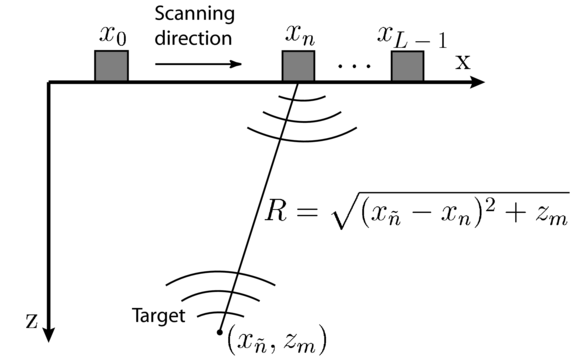
More specifically, to achieve focus at an observation point , the SAFT algorithm time shifts and performs a summation of the received signals measured at transducer positions for all in the synthetic aperture. The time shifts which aim to compensate for differences in pulse traveling time, are simply calculated using the Pythagorean theorem and the operation is commonly expressed in the continuous time form [15]
| (16) |
where is the beamformed image.
The DREAM Toolbox has two functions saft and saft_p, respectively, that performs the SAFT operation (with linear interpolation):
Input parameters:
The SAFT method described in Section 11.2 is a special case of methods based on so-called delay-and-sum imaging (DAS). The simple idea is just to compensate for the double-path propagation delay from each transmitter/receiver to each observation point and then perform a (coherent) summation. This operation is essentially based on an geometrical optics approach and is analogous to the operation of an acoustical lens [16].
The DREAM Toolbox has two functions to facilitate (matrix based) delay-and-sum processing. The two DAS functions das and das_arr is similar to the transducer functions in the sense that they return a matrix with responses corresponding to each observation point. The difference from the transducer functions is that only the time delay is computed which is represented with a “1” at the corresponding index.
The das function is for single transducers and the das_arr function is for arrays. The input parameters,
are similar to the ones used in the transducer functions previously described.
In this section a short introduction to model based ultrasonic imaging is presented. Model based ultrasonic array imaging [17–19] is different from delay-and-sum imaging in the sense that is based on optimal information processing whereas delay-and-sum imaging is based on geometrical focusing. The idea is to use a (linear) model, taking into account the diffraction effects associated with each transmitter/receiver, the electrical characteristics for each transmitter/receiver, as well as the used input signal(s), and then estimate the parameters (the scattering strengths) of the model based on both data and prior information. The DREAM toolbox can be used in this process for computing the SIRs for the model which can then be convolved with measured electrical impulse responses to obtain a model for a real measurement setup or using only simulated impulse responses to evaluate different array designs, for example.
To obtain a linear mode we need to consider both the forward process and the backward process. As discussed in Section 5.1 [Eq. (2)] the forward response can be divided in three parts: the input signal , the forward electro-acoustical response , and the forward SIR . The backward response can similarly be divided in two parts: the backward acousto-electrical impulse response and the backward SIR . Now, consider an array with transmit elements and receive elements and contributions from a single observation point, , where denotes the transpose operator. The received signal, , from the th receive element can be expressed
| (17) |
where denotes temporal convolution and is the noise for the th receive element. Note that the total forward impulse response is a superposition of the forward impulse responses corresponding to all transmit elements. The object function is the scattering strength at the observation point , is the forward electrical impulse response for the th transmit element, the backward electrical impulse response for the th receive element, and is the input signal for the th transmit element.
A discrete-time version of (15) is obtained by sampling the impulse responses and by using discrete-time convolutions. If we consider observation points then the received discrete waveform from a target at the th observation point, , can be expressed as
| (18) |
where the column vector is the discrete system impulse response for the th receive element.11 The vector represents the scattering amplitudes in the region-of-interest, and the notation denotes the th element in .12
To obtain the received signal for all observation points we need to perform a summation over , which equivalently can be expressed as a matrix-vector multiplication, according to
| (19) |
which gives us a liner model for the data for one receive element.
To obtain a model for all elements we can append all receive signals into a single vector and we finally have linear model for the total array setup
| (20) |
for the total array imaging system [20]. The propagation matrix, , in (20) now describes both the transmission and the reception process for an arbitrary focused array. Note that the position of the observation points, and the corresponding scattering amplitudes represented by the vector , is not restricted to a regular two-dimensional grid, which is often used in ultrasonic imaging. Furthermore, the array elements can in fact, similar to the observation points , be positioned at arbitrary locations in tree-dimensional space space. Thus, the model (20) can also be used to model two-dimensional arrays as well as to model array responses in tree-dimensional space. Also note that the “noise” vector describes the uncertainty of the model (20). The noise does not only model the measurement noise but also all other errors that we may have, such as: multiple scattering effects, cross talk between array elements, non-uniform sound speed in the media, etc.
The matched filter has the property of maximizing the signal-to-noise ratio (at a single point). The matched filter for each observation point is given by [18]
| (21) |
Note that the structure of the matched filter is similar to delay-and-sum processing which also can be expressed as a matrix-vector multiplication (see the model_based_example.m on the DREAM website),
| (22) |
where the delay matrix has ones in the positions corresponding the the propagation delays and zeros otherwise.
The optimal linear estimator (or the Wiener filter) is given by [17, 19]
| (23) |
where is the covariance matrix for and is the covariance matrix for , respectively. The estimator (23) has the property, not found for the matched filter or for delay-and-sum methods, namely that any beampattern can be compensated given that the signal-to-noise ratio is sufficient.
As a final not on model based imaging is that the matrices involved normally become rather large. It is therefore highly recommended to used a tuned linear algebra library, such as K. Goto’s BLAS library or the ATLAS library, for example. These libraries often have thread support so that all CPUs on the computer can be utilized.
An example of model based (and matrix based delay-and-sum) imaging can be found on the DREAM website (see the model_base_example.m file on the examples page).
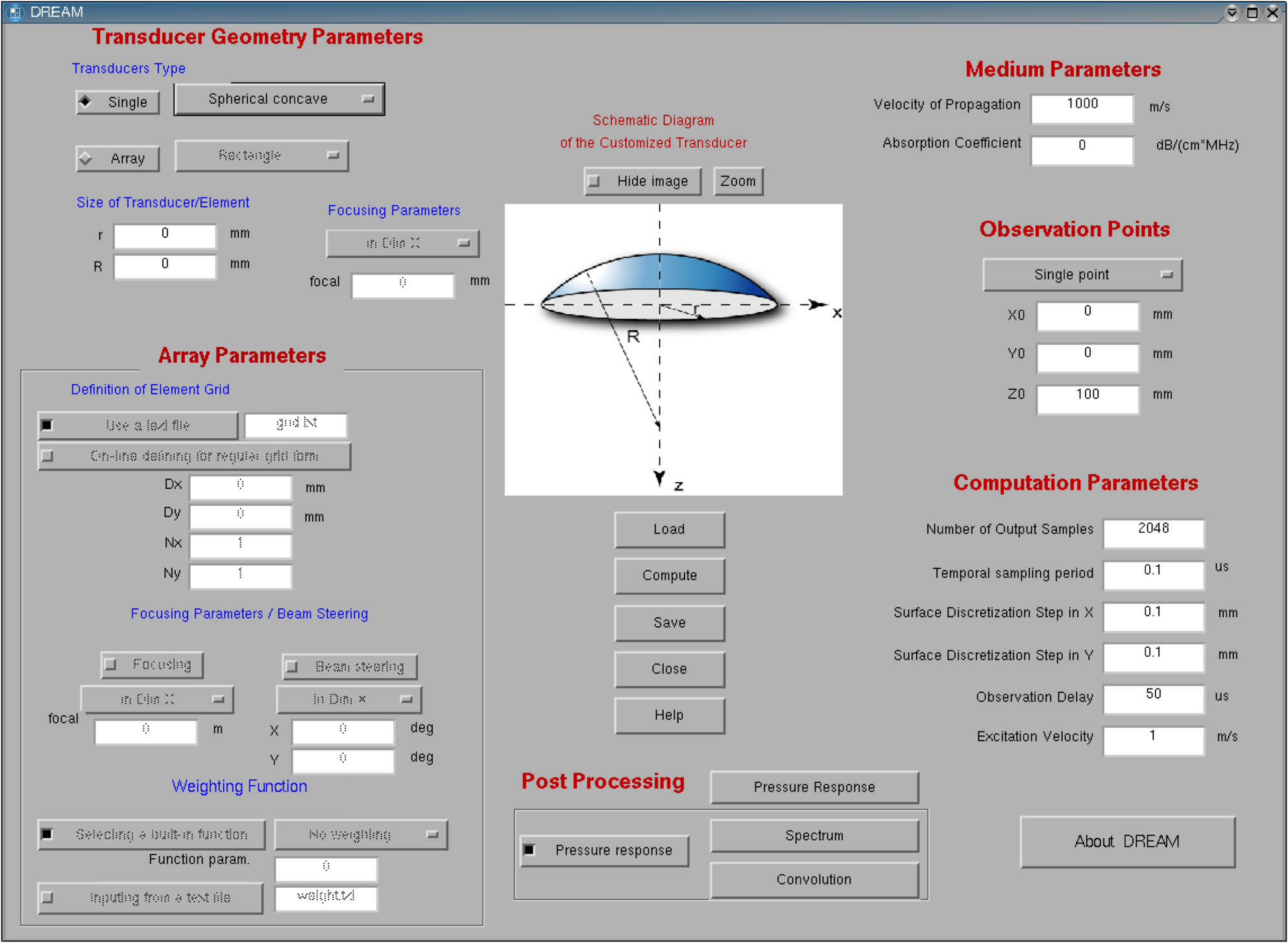
To launch the DREAM Toolbox GUI, type dream_gui in the Matlab Command Window and a graphical user interface will be raised as shown in Figure 9.
After activating the user interface, users can set parameters, compute SIRs, and save and process the resulting SIR by using the graphical controls. For setting of geometry parameters, please also refer to the schematic diagram of transducer displayed in the center of the graphic interface. After setting all the parameters, clicking on the Compute button starts to compute SIR. In addition, the DREAM GUI provides several post-processing operations to process the SIRs, including computing pressure response, computing the spectrum of the SIR, and convolving the SIR with an excitation signal. Notice that if users tick the checkbox of pressure response, the spectrum and convolution operations will be performed on the pressure instead of on the SIR. The parameters and resulting SIR can be stored in an *.mat file by clicking on the button of Save. The parameters settings can then be restored by loading the file using the Load button.
or rename matlab/sys/os/glnx86/libgcc_s.so and copy (or link) a working libgcc_s.so to the matlab/sys/os/glnx86/ directory.
[1] B. Piwakowski and B. Delannoy, “Method for computing spatial pulse response: Time-domain approach”, J. Acoust. Soc. America 86, 2422–32 (1989).
[2] B. Piwakowski and K. Sbai, “A new approach to calculate the field radiated from arbitrarily structured transducer arrays”, IEEE Transactions on Ultrasonics, Ferroelectrics and Frequency Control 46, 422–40 (1999).
[3] G. E. Tupholme, “Generation of acoustic pulses by baffled plane pistons”, Mathematika 16, 209–224 (1969).
[4] P. Stepanishen, “Transient radiation fom pistons in an infinite planar baffle”, J. Acoust. Soc. America 49, 1629–38 (1971).
[5] K. Aki and P. Richards, Quantitative Seismology (W.H. Freeman, San Francisco) (1980).
[6] J. Lockwood and J. Willette, “High-speed method for computing the exact solution for the pressure variations in the nearfield of a baffled piston”, J. Acoust. Soc. America 53, 735–741 (1973).
[7] http://www.fftw.org.
[8] V. A. Del Grosso, “New equation for the speed of sound in natural waters (with comparisons to other equations)”, J. Acoust. Soc. America 56, 1084–109 (1974).
[9] P. Stepanishen, “Pulsed transmit/receive response of ultrasonic piezoelectric transducers”, J. Acoust. Soc. America 69, 1815–1827 (1981).
[10] C. Wiley, “Synthetic aperture radars”, IEEE Trans. on Aerosp. Electron. Syst. 21, 440–443 (1985).
[11] C. Sherwin, J. Ruina, and R. Rawcliffe, “Some early developments in synthetic aperture radar systems”, IRE Trans. Military Electron. 6, 111–115 (1962).
[12] P. Gough and D. Hawkins, “Imaging algorithms for strip-map synthetic aperture sonar: Minimizing the effects of aperure errors and aperture undersampling”, IEEE Journal of Oceanic Engineering 22, 27–39 (1997).
[13] J. Seydel, “Ultrasonic synthetic-aperture focusing techniques in NDT”, Research Techniques for Nondestructive Testing (Academic Press) (1982).
[14] S. Doctor, T. Hall, and L. Reid, “SAFT—the evolution of a signal processing technology for ultrasonic testing”, NDT International 19, 163–172 (1986).
[15] C. Frazier and J. W.D. O’Brien, “Synthetic aperture techniques with a virtual source element”, IEEE Transactions on Ultrasonics, Ferroelectrics, and Frequency Control 45, 196–207 (1998).
[16] G. S. Kino, Acoustic Waves: Devices, Imaging and Analog Signal Processing, volume 6 of Prentice-Hall Signal Processing Series (Prentice-Hall) (1987).
[17] R. Stoughton, “Source imaging with minimum mean-squared error”, jasa 94, 827–834 (1993).
[18] F. Lingvall, T. Olofsson, and T. Stepinski, “Synthetic aperture imaging using sources with finite aperture: Deconvolution of the spatial impulse response”, J. Acoust. Soc. America 114, 225–234 (2003).
[19] F. Lingvall and T. Olofsson, “On time-domain model based ultrasonic array imaging”, 54, 1623–1633 (2007).
[20] F. Lingvall, “A method of improving overall resolution in ultrasonic array imaging using spatio-temporal deconvolution”, Ultrasonics 42, 961–968 (2004).
The DREAM toolbox uses pthreads (POSIX threads) to run computations in parallel on several cores/cpus. To
run the parallel functions on Windows the Pthreads-win32 library is used:
http://sourceware.org/pthreads-win32/. The most current version of the Pthreads-win32 library, which
is the one used by DREAM, is version 2.8.0 (2006-12-22). A 32-bit binary version of the library
can be found at: ftp://sourceware.org/pub/pthreads-win32/. The MinGW-w64 project has a
patch to build the Pthreads-win32 lib for 64-bit Windows, and there are some more 64-bit patches
at:
http://www.cadforte.com/wiki/index.php/Pthreads.
To facilite building the lib we have included our own (experimental) patch, which is a combination of the patches above (with some minor changes), and the source code for the Pthreads-win32 lib in the source code packge of the DREAM toolbox. There are also two (bash) build scripts which can be used for building the 32-bit and 64-bit libs, respectively. This is tested using the MinGW-w32 and MinGW-w64 cross compiler tool chains on Linux. After uncompressing the DREAM source code packge you can find these files in the windows folder.
Given that you have installed the MinGW-w32 cross compiler you can build the 32-bit Pthreads-win32 with
This will build the pthreadGC2.dll file and copy it (the pthread.def file, and the header files pthread.h, sched.h and, semaphore.h) to the windows/dll folder.
For 64-bit windows you first need to install the MinGW-w64 cross compiler and then the script
will copy the Pthreads-win32 sources, patch them for 64-bits support, and build the lib. The 64-bit lib (the pthread.def file, and the header files pthread.h, sched.h and, semaphore.h) will be installed in the windows/dll_64 folder.
Note: if you intend to use these libs with one of the MSVC compilers then you also need the corresponding lib files. These lib files can be generated using the windows bat-files found in the windows/dll and windows/dll_64 folders, respectively.
For conveniance we have also included the sources for the FFTW library and two scripts to build the library for both 32 and 64 bit Windows. The (bash) scripts uses MinGW-w32 and MinGW-w64 cross compiler tool chains, respectively. Change directory to the windows folder and run
to build for 32-bit Windows or
for 64-bit Windows. The two build scripts are based on the corresponding ones at the FFTW site adapted for building DREAM on Windows. The scripts install the libraries in the windows/dll and windows/dll_64 folders, respectively.
Similary to the Pthreads-win32 lib you need to build the lib files if you intend to use these libs with one of the MSVC compilers. These lib files can be generated using the corresponding windows bat-files found in the windows/dll and windows/dll_64 folders, respectively.